Originally posted on TowardsDataScience.
Table of Contents
- Preamble
- Neural Network Generalization
- Back to Basics: The Bayesian Approach
- How to Use a Posterior in Practice?
- Bayesian Deep Learning
- Back to the Paper
- Final Words
Preamble
Bayesian (deep) learning has always intrigued and intimidated me. Perhaps because it leans heavily on probabilistic theory, which can be daunting. I noticed that even though I knew basic probability theory, I had a hard time understanding and connecting that to modern Bayesian deep learning research. The aim of this blogpost is to bridge that gap and provide a comprehensive introduction.
Instead of starting with the basics, I will start with an incredible NeurIPS 2020 paper on Bayesian deep learning and generalization by Andrew Wilson and Pavel Izmailov (NYU) called Bayesian Deep Learning and a Probabilistic Perspective of Generalization. This paper serves as a tangible starting point in which we naturally encounter Bayesian concepts in the wild. I hope this makes the Bayesian perspective more concrete and speaks to its relevance.
I will start with the paper abstract and introduction to set the stage. As we encounter Bayesian concepts, I will zoom out to give a comprehensive overview with plenty of intuition, both from a probabilistic as well as ML/function approximation perspective. Finally, and throughout this entire post, I’ll circle back to and connect with the paper.
I hope you will walk away not only feeling at least slightly Bayesian, but also with an understanding of the paper’s numerous contributions, and generalization in general ;)
Neural Network Generalization (Abstract & Introduction)
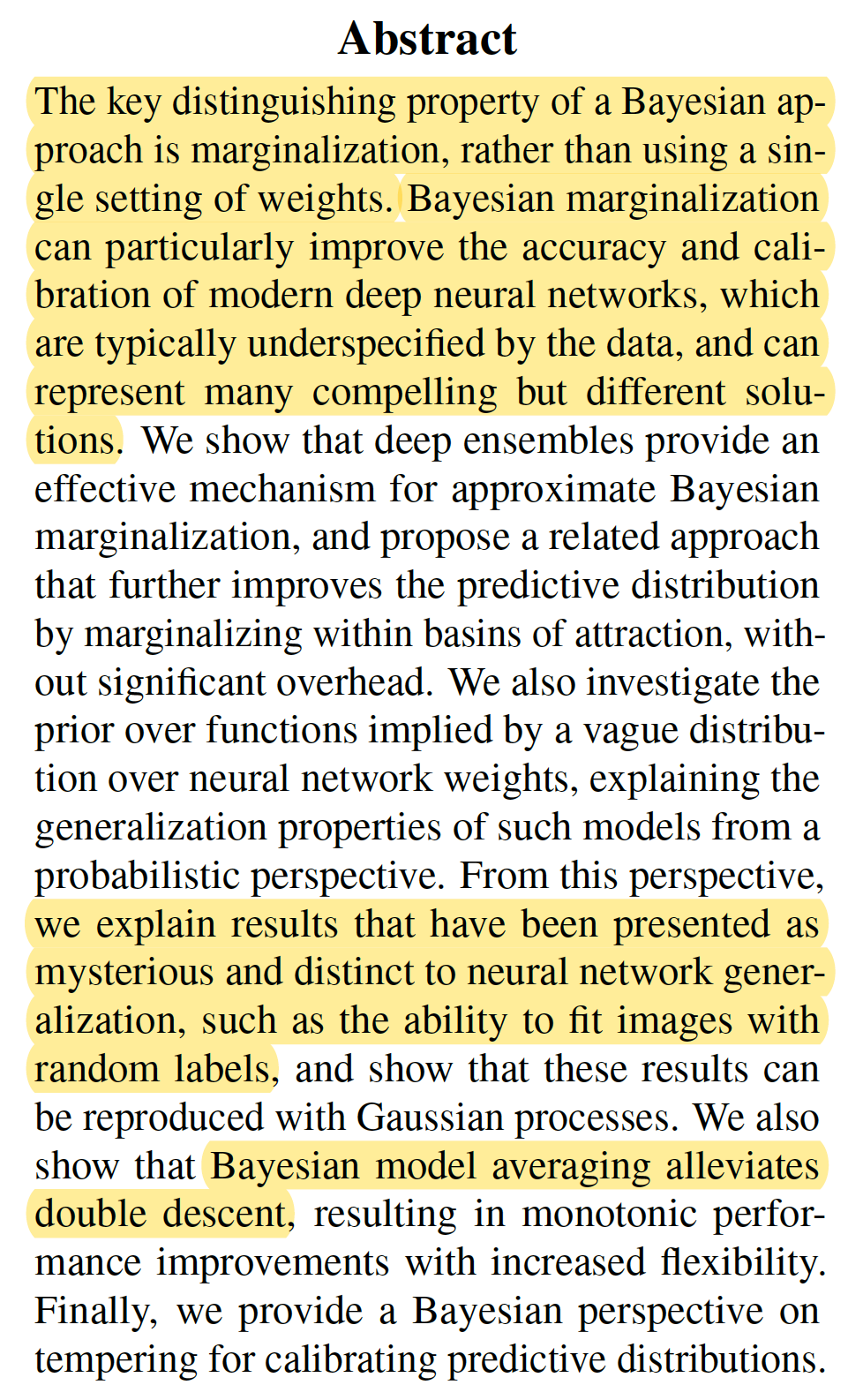
If your Bayesian is a bit rusty the abstract might seem rather cryptic. The first two sentences are of particular importance to our general understanding of Bayesian DL. The middle part presents three technical contributions. The last two highlighted sentences provide a primer on new insights into mysterious neural network phenomena. I’ll cover everything, but first things first: the paper’s introduction.
 |
|---|
| Abstract of “Bayesian Deep Learning and a Probabilistic Perspective of Generalization” by Andrew Wilson and Pavel Izmailov (NYU) |
An important question in the introduction is how and why neural networks generalize. The authors argue that
“From a probabilistic perspective, generalization depends largely on two properties, the support and the inductive biases of a model.”
Support is the range of dataset classes that a model can support. In other words; the range of functions a model can represent, where a function is trying to represent the data generative process. The inductive bias defines how good a model class is at fitting a specific dataset class (e.g. images, text, numerical features). The authors call this, quite nicely, the “distribution of support”. In other words, model class performance (~inductive bias) distributed over the range of all possible datasets (support).
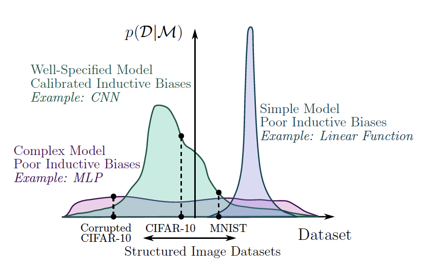
Let’s look at the examples the authors provide. A linear function has truncated support as it cannot even represent a quadratic function. An MLP is highly flexible but distributes its support across datasets too evenly to be interesting for many image datasets. A convolutional neural network exhibits a good balance between support and inductive bias for image recognition. Figure 2a illustrates this nicely.
 |
|---|
| Support and its distribution (inductive bias) for several model types. Wilsen et al. (2020) Figure 2a |
The vertical axis represents what I naively explained as “how good a model is at fitting a specific dataset”. It actually is Bayesian evidence, or marginal likelihood; our first Bayesian concept! We’ll dive into it in the next section. Let’s first finish our line of thought.
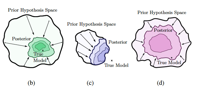
A good model not only needs a large support to be able to represent the true solution, but also the right inductive bias to actually arrive at that solution. The Bayesian posterior, think of it as our model for now, should contract to the right solution due to the right inductive bias. However, the prior hypothesis space should be broad enough such that the true model is functionally possible (broad support). The illustrations below (Figure 2 in the paper) demonstrate this for the three example models. From left to right we see a CNN in green, linear function in purple, and MLP in pink.
 |
|---|
| Relation between the prior, posterior and true model for model types with varying support and inductive bias. CNN (b), MLP (c) and linear model (d). Wilsen et al. (2020) Figure 2 |
At this point in the introduction, similar to first sentence of the abstract, the authors stress that
“The key distinguishing property of a Bayesian approach is marginalization instead of optimization, where we represent solutions given by all settings of parameters weighted by their posterior probabilities, rather than bet everything on a single setting of parameters.”
The time is ripe to dig into marginalization vs optimization, and broaden our general understanding of the Bayesian approach. We’ll touch on terms like the posterior, prior and predictive distribution, the marginal likelihood and bayesian evidence, bayesian model averaging, bayesian inference and more.
Back to Basics: The Bayesian Approach
We can find claims about marginalization being at the core of Bayesian statistics everywhere. Even in Bishop’s ML bible Pattern Recognition and Machine Learning (Chapter 3.4), but also here. The opposite to the Bayesian perspective is the frequentist perspective. This is what you encounter in most machine learning literature. It’s also easier to grasp. Let’s start there.
Frequentists
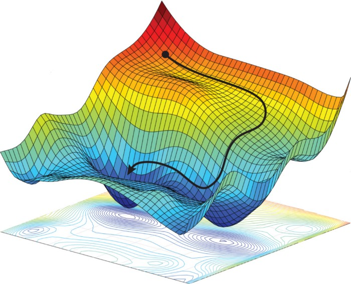
The frequentist approach to machine learning is to optimize a loss function to obtain an optimal setting of the model parameters. An example loss function is cross-entropy, used for classification tasks such as object detection or machine translation. The most commonly used optimization techniques are variations on (stochastic) gradient descent. In SGD the model parameters are iteratively updated in the direction of the steepest descent in loss space. This direction is determined by the gradient of the loss with respect to the parameters. The desired result is that for the same or similar inputs, this new parameter setting causes the output to closer represent the target value. In the case of neural networks, gradients are often computed using a computational trick called backpropagation.
 |
|---|
| Navigating a loss space in the direction of steepest descent using Gradient Descent. Amini et al. (2017) Figure 2. |
From a probabilistic perspective, frequentists are trying to maximize the likelihood \(p(\mathcal{D}|w, \mathcal{M})\). In plain english: to pick our parameters \(w\) such that they maximize the probability of the observed dataset \(\mathcal{D}\) given our choice of model \(\mathcal{M}\) (Bishop, Chapter 1.2.3). \(\mathcal{M}\) is often left out for simplicity. From a probabilistic perspective, a (statistical) model is simply a probability distribution over data \(\mathcal{D}\) (Bishop, Chapter 3.4). For example; a language model outputs a distribution over a vocabulary, indicating how likely each word is to be the next word. It turns out this frequentist way of maximum likelihood estimation (MLE) to obtain, or “train”, predictive models can be viewed from a larger Bayesian context. In fact, MLE can be considered a special case of maximum a posteriori estimation (MAP, which I’ll discuss shortly) using a uniform prior.
Bayesianists
A crucial property of the Bayesian approach is to realistically quantify uncertainty. This is vital in real world applications that require us to trust model predictions. So, instead of a parameter point estimate, a Bayesian approach defines a full probability distribution over parameters. We call this the posterior distribution. The posterior represents our belief/hypothesis/uncertainty about the value of each parameter (setting). We use Bayes’ Theorem to compute the posterior. This theorem lies at the heart of Bayesian ML - hence the name - and can be derived using simple rules of probability.
\[posterior = \frac{likelihood * prior}{evidence}, \;or \; p(w|\mathcal{D}) = \dfrac{p(\mathcal{D}|w)p(w)}{p(\mathcal{D})}\] \[evidence=p(\mathcal{D}) = \int p(\mathcal{D}|w)p(w)d w\]We start with specifying a prior distribution \(p(w)\) over the parameters to capture our belief about what our model parameters should look like prior to observing any data.
Then, using our dataset, we can update (multiply) our prior belief with the likelihood \(p(\mathcal{D}|w)\). This likelihood is the same quantity we saw in the frequentist approach. It tells us how well the observed data is explained by a specific parameter setting \(w\). In other words; how good our model is at fitting or generating that dataset. The likelihood is a function of our parameters \(w\).
To obtain a valid posterior probability distribution, however, the product between the likelihood and the prior must be evaluated for each parameter setting, and normalized. This means marginalizing (summing or integrating) over all parameter settings. The normalizing constant is called the Bayesian (model) evidence or marginal likelihood \(p(\mathcal{D})\).
These names are quite intuitive as \(p(D)\) provides evidence for how good our model (i.e. how likely the data) is as a whole. With “model as a whole” I mean taking into account all possible parameter settings. In other words: marginalizing over them. We sometimes explicitly include the model choice \(\mathcal{M}\) in the evidence as \(p(\mathcal{D}|\mathcal{M})\) . This enables us to compare different models with different parameter spaces. In fact, this comparison is exactly what happens in the paper when comparing the support and inductive bias between a CNN, MLP and linear model!
Bayesian Inference and Marginalization
We’ve now arrived at the core of the matter. Bayesian inference is the learning process of finding (inferring) the posterior distribution over \(w\). This contrasts with trying to find the optimal \(w\) using optimization through differentiation, the learning process for frequentists.
As we now know, to compute the full posterior we must marginalize over the whole parameter space. In practice this is often impossible (intractable) as we can have infinitely many such settings. This is why a Bayesian approach is fundamentally about marginalization instead of optimization.
The intractable integral in the posterior leads to a different family of methods to learn parameter values with. Instead of gradient descent, Bayesianists often uses sampling methods such as Markov Chain Monte Carlo (MCMC), or variational inference; techniques that try to mimic the posterior using a simpler, tractable family of distributions. Similar techniques are often used for generative models such as VAEs. A relatively new method to approximate a complex distribution is normalizing flows.
How to Use a Posterior in Practice?
Now that we understand the Bayesian posterior distribution, how do we actually use it in practice? What if we want to predict, say, the next word, let’s call it \(y\), given an unseen sentence \(x\)?
Maximum A Posteriori (MAP) Estimation
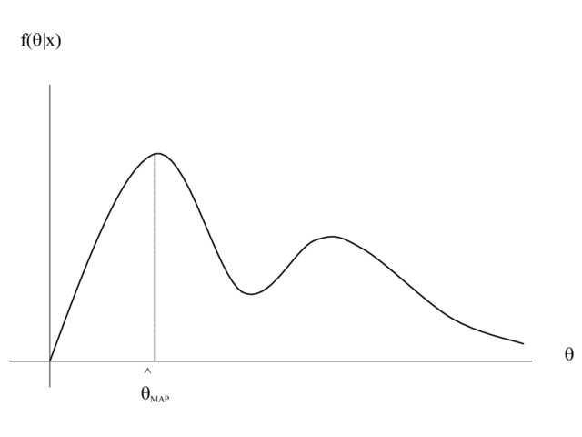
Well, we could simply take the posterior distribution over our parameters for our model \(\mathcal{M}\) and pick the parameter setting \(\hat{w}\) that has the highest probability assigned to it (the distribution’s mode). This method is called Maximum A Posteriori, or MAP estimation. But… It would be quite a waste to go through all this effort of computing a proper probability distribution over our parameters only to settle for another point estimate, right? (Except when nearly all of the posterior’s mass is centered around one point in parameter space). Because MAP provides a point estimate, it is not considered a full Bayesian treatment.
 |
|---|
| Maximum A Posteriori (MAP) estimation; not a full Bayesian treatment. Hero et al. (2008) Figure 17. |
Full Predictive Distribution
The full fledged Bayesian approach is to specify a predictive distribution \(p(y|\mathcal{D},x)\) .
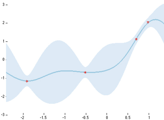
\[p(y|\mathcal{D}, x) = \int p(y|w, x)p(w|\mathcal{D})dw\]This defines the probability for class label \(y\) given new input \(x\) and dataset \(\mathcal{D}\). To compute the predictive distribution we need to marginalize over our parameter settings again! We multiply the posterior probability of each setting \(w\) with the probability of label \(y\) given input \(x\) using parameter setting \(w\). This is called Bayesian Model Averaging, or BMA; we take a weighted average over all possible models (parameter settings in this case). The predictive distribution is the second important place for marginalization in Bayesian ML, the first being the posterior computation itself. An intuitive way to visualize a predictive distribution is with a simple regression task, like in the Figure below. For a concrete example check out these slides (9-21).
 |
|---|
| Predictive distribution on a simple regression task. High certainty around observed data points; high uncertainty elsewhere. Yarin Gal (2015) |
Approximate Predictive Distribution
As we know by now, the integral in the predictive distribution is often intractable and at the very least extremely computationally expensive. A third method to using a posterior is by sampling a few parameters settings and combining the resulting models (e.g. approximate BMA). This is actually called a Monte Carlo approximation of the predictive distribution!
This last method is vaguely reminiscent of something perhaps more familiar to a humble frequentist: deep ensembles. Deep ensembles are formed by combining neural networks that are architecturally identical, but trained with different parameter initializations. This beautifully ties in with where we left off in the paper! Remember the abstract?
“We show that deep ensembles provide an effective mechanism for approximate Bayesian marginalization, and propose a related approach that further improves the predictive distribution by marginalizing within basins of attraction”.
Reading the abstract for the second time, the contributions should make a lot more sense. Also, we are now finally steering into Bayesian Deep Learning territory!
Bayesian Deep Learning
A Bayesian Neural Network (BNN) is simply posterior inference applied to a neural network architecture. To be precise, a prior distribution is specified for each weight and bias. Because of their huge parameter space, however, inferring the posterior is even more difficult than usual.
So why do Bayesian DL at all?
The classic answer is to obtain a realistic expression of uncertainty, or calibration. A classifier is considered calibrated if the probability (confidence) of a class prediction aligns with its misclassification rate. As said before, this is crucial in real world applications.
“Neural networks are often miscalibrated in the sense that their predictions are typically overconfident.”
However, Wilson and Izmailov, the authors of our running example paper, argue that Bayesian model averaging increases accuracy as well. According to Section 3.1, the Bayesian perspective is in fact especially compelling for neural networks! Because of their large parameter space, neural networks can represent many different solutions, e.g. they are underspecified by the data. This means a Bayesian model average is extremely useful because it combines a diverse range of functional forms, or “perspectives”, into one.
“A neural network can represent many models that are consistent with our observations. By selecting only one, in a classical procedure, we lose uncertainty when the models disagree for a test point.”
Recent Approaches To (Approximate) Bayesian Deep Learning
A number of people have recently been trying to combine the advantages of a traditional neural network (e.g. computationally efficient training using SGD & back propagation) with the advantages of a Bayesian approach (e.g. calibration).
Monte Carlo Dropout
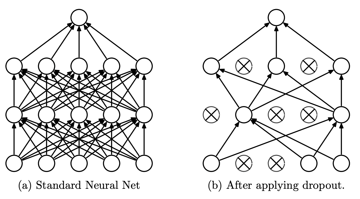
One popular and conceptually easy approach is Monte Carlo dropout. Recall that dropout is traditionally used as regularization; it provides stochasticity or variation in a neural network by randomly shutting down weights during training. It turns out dropout can be reinterpreted as approximate Bayesian inference and applied during testing, which leads to multiple different parameter settings. Sounds a little similar to sampling parameters from a posterior to approximate the predictive distribution, mh?
 |
|---|
| In the original dropout mechanism, some neurons are randomly shut down during training. Srivastava et al. (2014), Figure 1. |
Stochastic Weight Averaging - Gaussian (SWAG)
Another line of work follows from Stochastic Weight Averaging (SWA), an elegant approximation to ensembling that intelligently combines weights of the same network at different stages of training (check out this or this blogpost if you want to know more). SWA-Gaussian (SWAG) builds on it by approximating the shape (local geometry) of the posterior distribution using simple information provided by SGD. Recall that SGD “moves” through the parameter space looking for a (local) optimum in loss space. To approximate the local geometry of the posterior, they fit a Gaussian distribution to the first and second moment of the SGD iterate. Moments describe the shape of a function or distribution, where the zero moment is the the sum, the first moment is the mean, and the second moment is the variance. These fitted Gaussian distributions can then be used for BMA.
Frequentist Alternatives to Uncertainty Representation
I have obviously failed to mention at least 99% of the field here (e.g. KFAC Laplace and temperature scaling for improved calibration), and picked the examples above in part because they are related to our running paper. I’ll finish with one last example of a recent frequentist (or is it…) alternative to uncertainty approximation. This is an often cited method that shows you can train a deep ensemble and use it to form a predictive distribution, resulting in a well calibrated model. They use a few bells and whistles that I won’t go into, such as adversarial training to smoothen the predictive distribution. Check out the paper here.
Back to the Paper
By now we are more than ready to circle back to the paper and go over its contributions! They should be easier to grasp :)
Deep Ensembles are BMA (Section 3)
Contrary to how recent literature (myself included) has framed it, Wilson and Izmailov argue that deep ensembles are not a frequentist alternative to obtain Bayesian advantages. In fact, they are a very good approximation of the posterior distribution. Because deep ensembles are formed by MAP or MLE retraining, they can form different basins of attraction. A basin of attraction is a “basin” or valley in the loss landscape that leads to some (locally) optimal solution. But there might be, and usually are, multiple optimal solutions, or valleys in the loss landscape. The use of multiple basins of attraction, found by different parts of an ensemble, results in more functional diversity than Bayesian approaches that focus on approximating posterior within single basin of attraction.
Combining Deep Ensembles with Bayesian Neural Networks (Section 4)
This idea of using multiple basins of attraction is important for the next contribution as well: an improved method for approximating predictive distributions. By combining the multiple basins of attraction property that deep ensembles have with the Bayesian treatment in SWAG, the authors propose a best-of-both-worlds solution: Multiple basins of attraction Stochastic Weight Averaging Gaussian or MultiSWAG:
“MultiSWAG combines multiple independently trained SWAG approximations, to create a mixture of Gaussians approximation to the posterior, with each Gaussian centred on a different basin. We note that MultiSWAG does not require any additional training time over standard deep ensembles.”
Have a look at the paper if you’re interested in the nitty gritty details ;)
Neural Network Priors (Section 5)
How can we ever specify a meaningful prior over millions of parameters, I hear you ask? It turns out this is a pretty valid question. In fact, the Bayesian approach is sometimes criticised because of it.
However, in Section 5 of the paper Wilson and Izmailov provide evidence that specifying a vague prior, such as a simple Gaussian might actually not be such a bad idea.
“Vague Gaussian priors over parameters, when combined with a neural network architecture, induce a distribution over functions with useful inductive biases.”
“The distribution over functions controls the generalization properties of the model; the prior over parameters, in isolation, has no meaning.”
A vague prior combined with the functional form of a neural network results in a meaningful distribution in function space. The prior itself doesn’t matter, but its effect on the resulting predictive distribution does.
Rethinking Generalization & Double Descent (Section 6 and 7)
We have now arrived at the strange neural network phenomena I highlighted in the abstract. According to Section 6, the surprising fact that neural networks can fit random labels is actually not surprising at all. Not if you look at it from perspective of support and inductive bias. Broad support, the range of datasets for which \(p(D|\mathcal{M}) > 0\) , is important for generalization. In fact, the ability to fit random labels is perfectly fine as long as we have the right inductive bias to steer the model towards a good solution. Wilson and Izmailov also show that this phenomena is not mysteriously specific to neural networks either, and that Gaussian Processes exhibit the same ability.
Double Descent
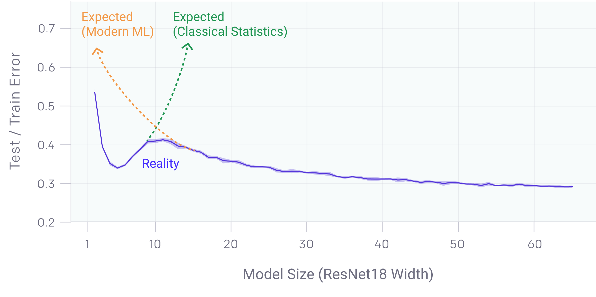
The second phenomena is double descent. Double descent is a recently discovered phenomena where bigger models and more data unexpectedly decreases performance.
 |
|---|
| This Figure is taken from this OpenAI blogpost that explains Deep Double Descent |
Wilson and Izmailov find that models trained with SGD suffer from double descent, but that SWAG reduces it. More importantly, both MultiSWAG as well as deep ensembles completely mitigate the double descent phenomena! This is in line with their previously discussed claim that
“Deep ensembles provide a better approximation to the Bayesian predictive distribution than conventional single-basin Bayesian marginalization procedures.”
and highlights the importance of marginalization over multiple modes of the posterior.
Final Words
You made it! Thank you for reading all the way through. This post became quite lengthy but I hope you learned a lot about Bayesian DL. I sure did.
Note that I am not affiliated to Wilson, Izmailov or their group at NYU. This post reflects my own interpretation of their work, except for the quote blocks taken directly from the paper.
Please feel free to ask any question or point out mistakes that I’ve undoubtedly made. I would also love to know whether you liked this post. You can find my contact details below and message me on Twitter and connect on LinkedIn.